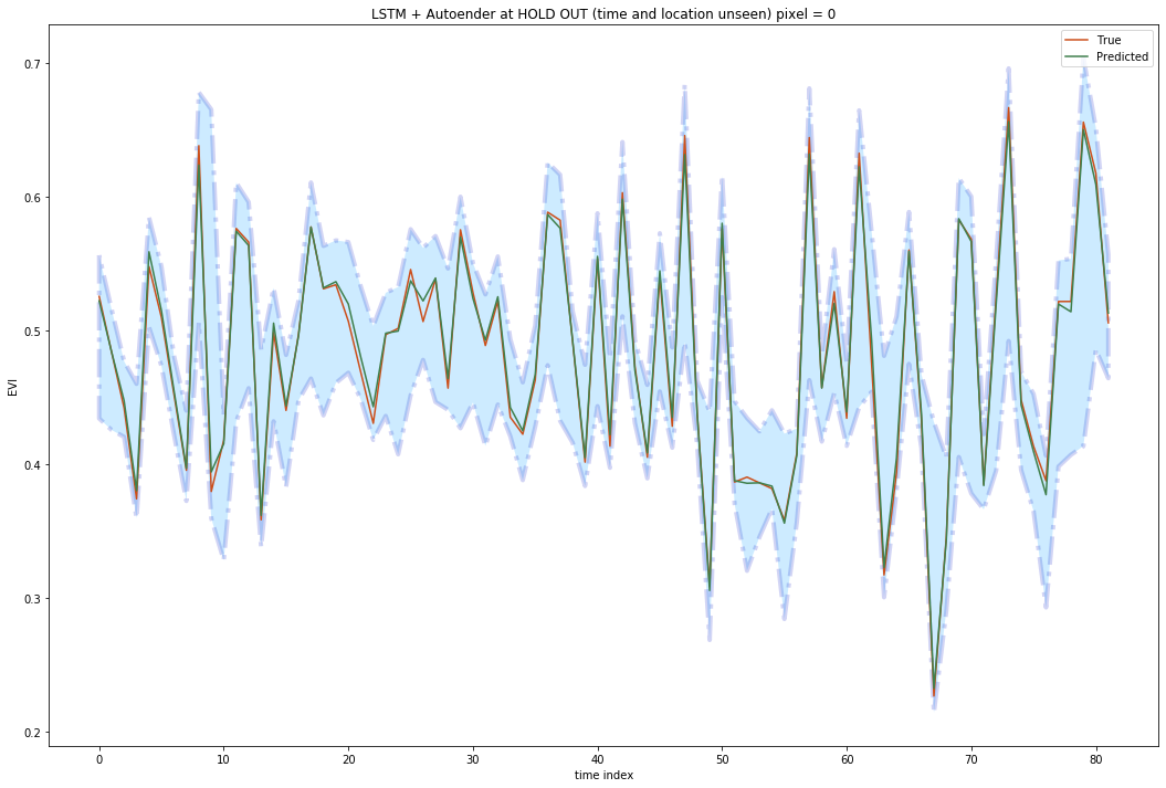
Bayesian Uncertainty for time series data (EVI) prediction using LSTM and autoencoder

Introduction
Bayesian NN
How much confidence do you know about your model results or a paritcular prediction?
This is a critical important question for many business. With the advent of deep learning, many forecasting problems for business have been solved in innovative ways. For example, Uber researchers has provided a fascianting paper on time series prediction.
Standard deep learning method such as LSTM do not capture model uncertianty. However, the uncertianty estimation is indispensable for deep learning models.
Bayesian probability theory offers us mathematically grounded tools to reason about model uncertainty, but these usually come with a prohibitive computational cost [2].
In deep learning, there are two kinds of strategries to quantify the uncertianty: (1) MC dropout and (2) variational inference.
(1) Regarding MC dropout, Gal developed a framework casting dropout training in deep neural networks (NNs) as approximate Bayesian inference in deep Gaussian processes. This method can mitigates the problem of representing model uncertainty in deep learning without sacrificing either computational complexity or test accuracy.
(2)Variational inference such as sampling-based variational inference and stochastic variational inference has been applied to deep learning models, which have performed as well as dropout. However, this approach comes with a prohibitive computational cost. To represent uncertainty, the number of parameters in these appraoches is doubled for the same network size. Further, they require more time to converge and do not improve on existing techniques. Given that good uncertainty estimates can be cheaply obtained from common dropout models, this might result in unnecessary additional computation.
what is variational inference? In short, variational inference is an approach of approximating model posterior which would otherwise be difficult to work with directly. Intuitively, this is a measure of similarity between the two distributions although it is not symmetric. So minimising this objective fits our approximating distribution to the distribution we care about.
This is standard in variational inference where we fit distributions rather than parameters, resulting in our robustness to over-fitting.
How dropout to represent Bayesian approximation
Compared to standard NN, the BNN added a binary vector in each layer. We sample new realisations for the binary vectors bi for every input point and every forward pass thorough the model (evaluating the model’s output), and use the same values in the backward pass (propagating the derivatives to the parameters to be optimised W1,W2,b). The elements of vector bi take value 1 with probability 0≤pi≤1 for i=1,2…l. i is the ith layer.
The dropped weights b1W1 and b2W2 are often scaled by 1/pi to maintain constant output magnitude. At test time we do not sample any variables and simply use the full weights matrices W1,W2,b.
Actually, the dropout network is similar to a Gaussian process approximation. Different network structures and different non-linearities would correspond to different prior beliefs as to what we expect our uncertainty to look like. This property is shared with the Gaussian process as well. Different Gaussian process covariance functions would result in different uncertainty estimates. If you are interested in more details on the BNN. Please refer to [here](http://mlg.eng.cam.ac.uk/yarin/blog_3d801aa532c1ce.html) - Why Does It Even Make Sense?
Calculating prediction uncertainty with BNNs developed by Uber
The variance quantifies the prediction uncertainty, which can be broken down using the law of total variance. An underlying assumption for the model uncertainty equation is that yhat is generated by the same procedure, but this is not always the case. In anomaly detection, for instance, it is expected that certain time series will have patterns that differ greatly from the trained model. Therefore, reseachers from Uber propose that a complete measurement of prediction uncertainty should be composed of three parts:
1 model uncertainty
2 model misspecification
3 inherent noise level.
1 Model Uncertainty
Model uncertainty, also referred to as epistemic uncertainty, captures our ignorance of the model parameters and can be reduced as more samples are collected. The key to estimating model uncertainty is the posterior distribution , also referred to as Bayesian inference. This is particularly challenging in neural networks because of the non-conjugacy often caused by nonlinearities.
Here we used Monte Carlo dropout to approximate model uncertainty.
2 Model misspecification
Model misspecification captures the scenario where testing samples come from a different population than the training set, which is often the case in time series anomaly detection. Similar concepts have gained attention in deep learning under the concept of adversarial examples in computer vision, but its implication in prediction uncertainty remains relatively unexplored
Here we first fit a latent embedding space for all training time series using an encoder-decoder framework. From there, we are able to measure the distance between test cases and training samples in the embedded space.
After estimating uncertaitny from model misspecification, we combined model uncertianty with model misspecification uncertianty by connecting the encoder-decoder network with a prediction network, and treat them as one large network during inference.
3 Inherent noise
Inherent noise is mainly to capture the uncertainty in the data generation process and which is irreducible. Uber reseachers propose a simple but adaptive approach by estimating the noise level via the residual sum of squares, evaluated on an independent held-out validation set.
If you are interested in technical parts on these three sections, you can go to here for more details.
Project link: https://github.com/tankwin08/Bayesian_uncertainty_LSTM